Sioux Falls - User Equilibrium

1. Imports and data readin

First we load the paminco package and read the SiouxFalls data. The data was taken from here and converted to our format of choice: XML. The data for SiouxFalls comes with paminco and can be easily loaded:

import paminco

sioux = paminco.load_sioux()

By default the edge cost equal the link travel time: \(F_e = l_e\). The link travel time is defined as \begin{equation*} l_e(x_e) = \text{fft}_e \cdot \left( 1 + B_e \cdot \left(\frac{x}{\text{cap}_e}\right) ^ {p_e} \right) \end{equation*}

2. Calculating the user equilibrium flow with Frank-Wolfe

Now we can use the Frank-Wolfe optimizer to find an approximate minimum cost flow that conincides < with the user equilibrium. To achive this, we have to integrate the edge costs by: \begin{equation*} F_e = \int_0^{x_e} l_e(s) ds \end{equation*}

sioux.integrate_cost()
fw = paminco.NetworkFW(sioux)
fw.run(max_iter=200)

The UE flow can be accessed by:

fw.flow

array([ 4498.78057097,  8117.75415054,  4520.8817098 ,  5963.651268  ,
        8095.65301171, 14084.00744695, 10078.58505075, 14084.84185857,
       18072.92157057,  5258.05356586, 18090.17765647,  8796.49997698,
       15810.16647779,  5985.75240684,  8803.0964337 , 12496.14294718,
       12097.35243389, 15812.91126577, 12524.84054273, 12044.54569007,
        6876.52997473,  8388.35494491, 15820.82610697,  6835.85388815,
       21763.45935771, 21833.44290031, 17730.87544595, 23166.83390325,
       11030.00029716,  8101.45295276,  5341.63189158, 17598.38770266,
        8387.478704  ,  9767.80609638, 10055.6495003 ,  8402.3646957 ,
       12369.458678  , 12461.40911924, 11113.02280201,  9804.01068712,
        9055.42182028,  8392.29551274, 23226.33191814,  9096.21251962,
       19096.44965674, 18380.70282795,  8404.92188323, 11069.26575521,
       11664.75357145, 15305.66555632,  8105.16076571, 11652.60944729,
        9953.27008428, 15865.71800959, 15373.64207684, 19024.00206496,
       19127.82428331,  9944.83377308,  8672.78303267, 19044.7853293 ,
        8695.72134804,  6311.43911073,  7008.76207499,  6247.61940062,
        8625.02284511, 10300.44803092, 18349.6169156 ,  7016.30336481,
        8609.49424049,  9629.83826182,  8387.70940414,  9590.76503467,
        7884.39343104, 11104.97324326, 10252.15692544,  7840.73409529])

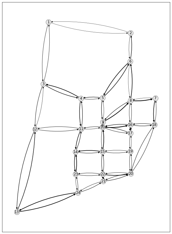
3. Plotting with NetworkX

Now we use the plotting capabilities of network to plot the equilibrium flow.

First, we build a nx.DiGraph from out network:

import matplotlib.pyplot as plt
import networkx as nx

# Get edgelist (pd.DataFrame) and pos dict
edgelist = sioux.get_flow_df(fw.flow)
pos = sioux.get_node_pos()

# Select only edge with flow
edgelist = edgelist[edgelist.flow > 0].reset_index()
G = nx.from_pandas_edgelist(
    edgelist,
    edge_attr=["flow"],
    create_using=nx.DiGraph(),
)

We setup a canves and plot the nodes (with labels) and the user equilibrium flow:

plt.figure(figsize=(10, 14))
nx.draw_networkx_nodes(G, pos, node_color="lightgrey", edgecolors="black", alpha=0.5)
nx.draw_networkx_edges(
    G, 
    pos, 
    width=2*edgelist.flow/edgelist.flow.max() + 0.2,
    connectionstyle="arc3, rad=0.1"
)
_  = nx.draw_networkx_labels(G, pos)