Setting up a Demand Function

1. Why do we need it?

paminco allows to compute parametric minimum cost flows (MCF) w.r.t. to demand multiplier \(\lambda\). I.e., the goal is to find a MCF for all values of \(\lambda\) in the interval \(\left[0, \lambda^{\max }\right]\):

\[\begin{split} \begin{align*} \min \text { } & C(\mathbf{x}) \\ \text {s.t.} \quad \mathbf{\Gamma} \mathbf{x} &= \mathbf{h}(\lambda), \\ \mathbf{x} &\geq \mathbf{0}, \end{align*} \end{split}\]

where \(\mathbf{h}(\lambda)\) is a demand function that maps \(\lambda\) to a demand vector \(\mathbf{b}\).

2. Demand vectors and matrices

2.1. Demand vector

For single commodity problems a demand vector is a (n, ) array that encodes the inflow and outflow rate per node, negative values indicating sources and positive values sinks.

Consider the following example. The network consists of four vertices and five edges. We want to send 10 units from vertex \(A\) to vertex \(D\), indicated by the wiggly green arrow

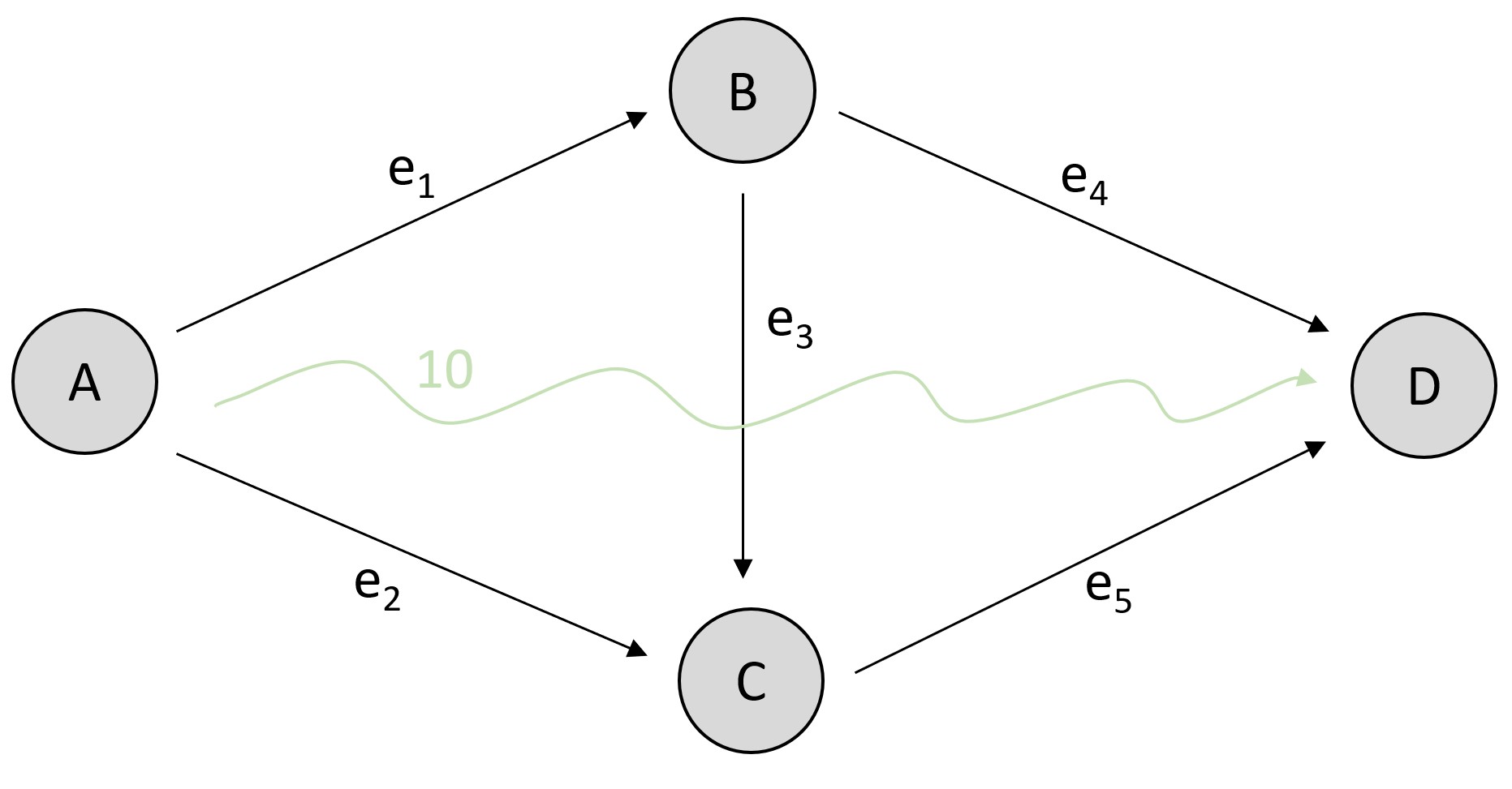
Simple network with demand.

Network setup

We setup this network (without demand) as follows:

import paminco
import numpy as np

edge_data = np.array([
    ["A", "B"],
    ["A", "C"],
    ["B", "C"],
    ["B", "D"],
    ["C", "D"],
])
graph = paminco.Network(edge_data)
graph.nodes.lbl2id

{'A': 0, 'B': 1, 'C': 2, 'D': 3}

Building demand vector

We now build a demand vector:

demand_vector = paminco.net.demand.demand_vector(
    ("A", "D", 10),  # send 10 units from A to D
    shared=graph.shared,  # each network element must know about shared data ...
)
demand_vector.map_node_label_to_id()

Retrieving sparse representation

This demand vector consists of one CommoditySingleSourceSink:

demand_vector.commodities

[CommoditySingleSourceSink @ 0x7f9eef43fbb0
 'A' (0) → 'D' (3) | 10.]

Algorithms in paminco expect the demand vector to be sparse matrix, which can be accessed by:

demand_vector()

<4x1 sparse matrix of type '<class 'numpy.float64'>'
	with 2 stored elements in Compressed Sparse Column format>

demand_vector().toarray()

array([[-10.],
       [  0.],
       [  0.],
       [ 10.]])

Setting demand function

We equip the network with a linear demand function that scales this demand vector by the demand multiplier \(\lambda\):

graph.set_demand(demand_vector)
graph.demand

<paminco.net.demand.LinearDemandFunction at 0x7f9eef43fdc0>

For a linear demand function with \(\lambda = 1\) (no scaling), we expect to retrieve the specified demand vector:

graph.demand(1).toarray()

array([[-10.],
       [  0.],
       [  0.],
       [ 10.]])

For other values of \(\lambda\), the input demand vector is scaled:

graph.demand(0.32).toarray()

array([[-3.2],
       [ 0. ],
       [ 0. ],
       [ 3.2]])

graph.demand(1.63).toarray()

array([[-16.3],
       [  0. ],
       [  0. ],
       [ 16.3]])

All in one go

By default, the network constructor builds a linear demand function from the demand_data:

graph.set_demand(("A", "D", 10))
graph.demand(1.63).toarray()

array([[-16.3],
       [  0. ],
       [  0. ],
       [ 16.3]])

2.2. Demand matrix

For certain problems, the demand may consist of multiple commodities. E.g., in a traffic network some drivers want to go from one location to another, and others vice versa. Consider an adaption of the graph above:

Demand as in/outflow per node in the graph.

Here, we set five commodities

\[\begin{split} \begin{align*} A & \overset{2}{\rightarrow} B \quad (\text{blue}), \\ A & \overset{5}{\rightarrow} D \quad (\text{orange}), \\ B & \overset{7}{\rightarrow} A \quad (\text{light green}), \\ C & \overset{5}{\rightarrow} B \quad (\text{dark green}), \\ D & \overset{5}{\rightarrow} C \quad (\text{red}). \end{align*} \end{split}\]

commodities = [
    ("A", "B", 2),
    ("A", "D", 5),
    ("B", "A", 7),
    ("C", "B", 5),
    ("D", "C", 5),
]
demand_matrix = paminco.net.demand_vector(commodities, shared=graph.shared)
demand_matrix.map_node_label_to_id()

We encoded the commodites in a demand matrix, where each column is a demand vector:

import pandas as pd
d = pd.DataFrame(demand_matrix().toarray())
d.set_index(graph.nodes.labels)

	0	1	2	3	4
A	-2.0	-5.0	7.0	0.0	0.0
B	2.0	0.0	-7.0	5.0	0.0
C	0.0	0.0	0.0	-5.0	5.0
D	0.0	5.0	0.0	0.0	-5.0

2.3. Commodity with multiple sinks and sources

So far, we considered only commodities that have a single source and single sink. However, for certain applications – such as a gas network – a commodity may consits of multiple sources and/or multiple sinks. This CommodityMultiSourceSink is encoded as a vector or dictionary that specfiies in and outflow rate of each node:

com = {"A": -5, "B": -2, "C": 1, "D": 6}
demand_vector = paminco.net.demand_vector(com, shared=graph.shared)
demand_vector.commodities

[CommodityMultiSourceSink @ 0x7f9eef43faf0
 'A' : -5.0
 'B' : -2.0
 'C' : 1.0
 'D' : 6.0]

In a sense, hhis commodity specifies that we input 5 units at \(A\) and 2 at \(B\), which are consumed by \(D (6)\) and \(C (1)\), i.e., \((A, B) \overset{7}{\rightarrow} (C, D)\).’

3. Function types

paminco has allows for two demand function types (other can be implemented by inheritance of paminco.demand.DemandFunction): linear demand functions and affine demand functions. For notational simplicity, we only consider demands that consists of a single commodity for the rest of this section.

3.1. Linear demand function

A linear demand function is of the form:

\[ \begin{equation} \mathbf{h}_{\text{lin}}(\lambda) = \lambda \mathbf{b}, \end{equation} \]

where \(\mathbf{b}\) is a demand vector (see 1.1). In a sense, the demand is simply scaled by the parameter \(\lambda\).

import paminco
import numpy as np

edge_data = np.array([
    ["A", "B"],
    ["A", "C"],
    ["B", "C"],
    ["B", "D"],
    ["C", "D"],
])
demand_data = ("A", "D", 1)

graph = paminco.Network(edge_data, demand_data=demand_data)

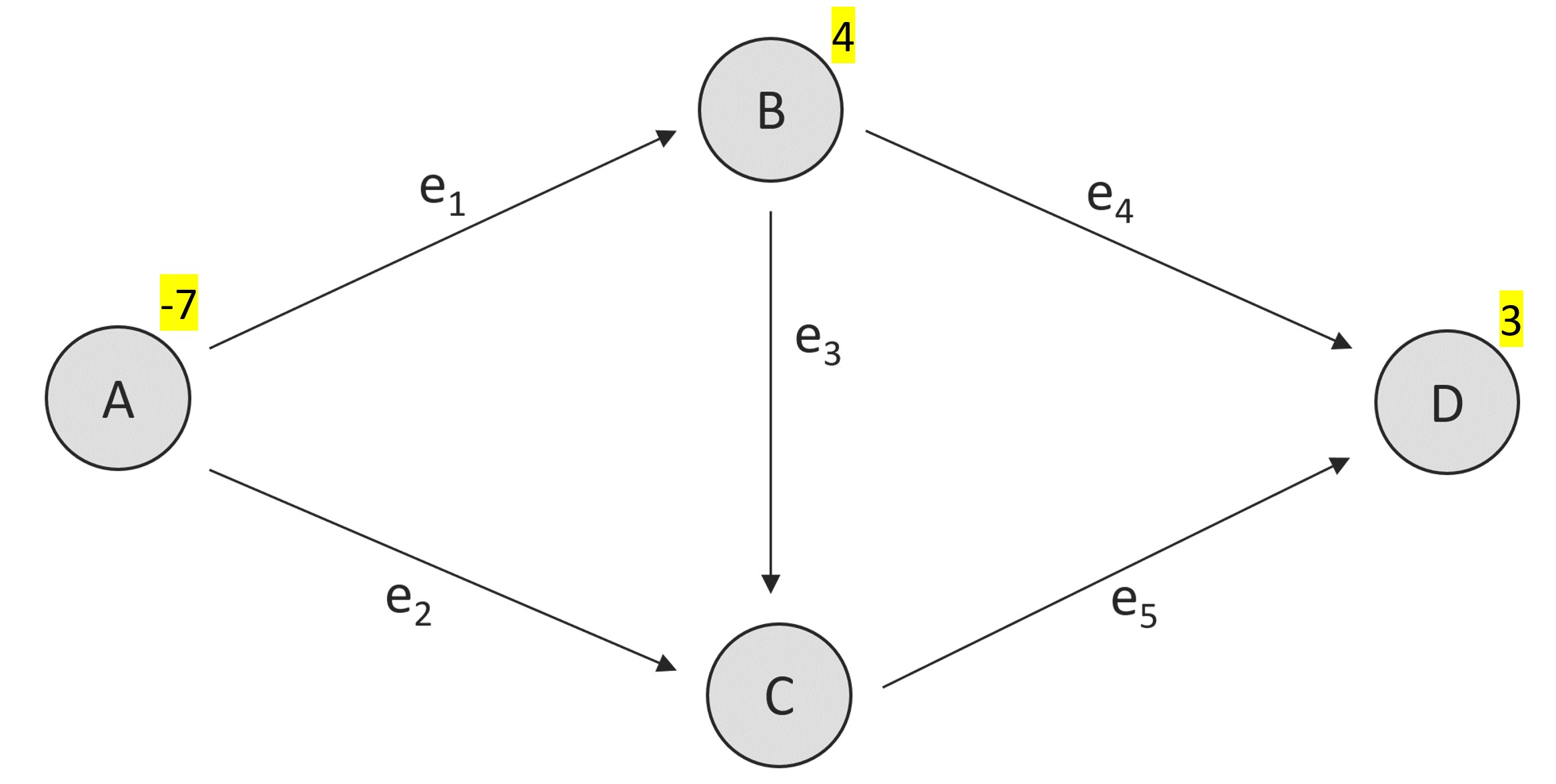
The demand function of the network for \(\lambda = 2.5\) – i.e., sending 2.5 times the original demand (1) from \(A\) to \(D\) – is called by:

graph.demand(2.5)   # or graph.h(2.5)

<4x1 sparse matrix of type '<class 'numpy.float64'>'
	with 2 stored elements in Compressed Sparse Column format>

which is a \(n \times k\) sparse matrix. This matrix encodes the in and outflow rates for all nodes (row) for all commodities (column). It is easily converted to a numpy.ndarray:

graph.demand(2.5).toarray()

array([[-2.5],
       [ 0. ],
       [ 0. ],
       [ 2.5]])

For example, the -2.5 indicates that the node at index 0 (node \(A\)) has a total inflow of -2.5 units, negative rates thus marking source. All the inflow in node \(A\) is then “consumed” by the node at index 3 (node \(D\), a sink).

3.2. Affine demand function

In contrast, an affine demand function consists of two parts: a base demand \(\mathbf{b}_0\) that is invariant of \(\lambda\) and a part that scales linearly with the demand multiplier:

\[ \begin{equation} \mathbf{h}_{\text{affine}}(\lambda) = \mathbf{b}_0 + \lambda \mathbf{b}. \end{equation} \]

This is of interest for problems where there exsists a trivial solution to problems with linearly scaled demands. Using the data from the above example, we can setup an affine demand function as follows:

b0 = ("B", "D", 1)
b = ("A", "D", 1)
demand_data = (b0, b)

graph2 = paminco.Network(
    edge_data, 
    demand_data=demand_data, 
    kw_demand={"mode": "affine"}
)

This graph now has a demand part that is independent of the demand multiplier:

graph2.h(0).toarray()

array([[ 0.],
       [-1.],
       [ 0.],
       [ 1.]])

and one that scales linearly with it:

graph2.h(7).toarray()

array([[-7.],
       [-1.],
       [ 0.],
       [ 8.]])

We can think of calling this affine demand function with \(\lambda = 7\) as sending 7 units from \(A\) to \(D\) and 1 unit from \(B\) to \(D\), resuilting in total 8 units in the sink \(D\).