Pigou’s Example

Consider the following network, also called Pigou’s example, where the two vertices s and t are connected with two parallel edges.

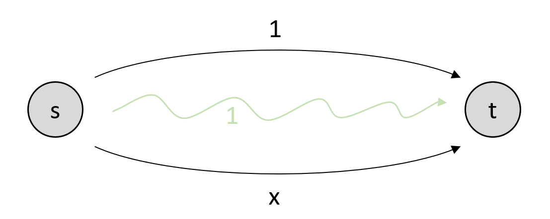
Pigou’s example.

The upper edge has a constant link travel time \(l_1(x_1) = 1\) invariant of the upper link flow \(x_1\), whereas the travel time on the lower edge varies by edge flow: \(l_2(x_2) = x_2\). In total, we send 1 unit from s to t, i.e., \(x_1\) is the fraction of driver that use the upper edge and \(x_2\) that use the lower edge, and \(x_1 + x_2 = 1\).

1. System optimum, user equilibrium and price of anarchy

1.1 System optimum (SO)

A centralized planner – e.g., the government – may strive to minimize the average travel time for all participants: \(\underset{\mathbf{x}}{\mathrm{argmin} \text{ }} \sum_{e \in E} x_{e} \cdot l_{e}(x_e)\).

The so called system optimum (SO) is easily computed by:

\[ \begin{equation*} \underset{x_1, x_2}{\mathrm{argmin} \text{ }} x_1 \cdot l_1(x_1) + x_2 \cdot l_2(x_2). \end{equation*} \]

By substituting \(x_2 = 1 - x_1\) this equals:

\[\begin{split} \begin{equation*} \underset{x_1}{\mathrm{argmin \text{ }}} x_1 \cdot 1 + (1-x_1) \cdot (1-x_1) = \\ \underset{x_1}{\mathrm{argmin \text{ }}} x_1 + (1-x_1)^2, \end{equation*} \end{split}\]

where the system optimal flow is: \(x_1 = x_2 = 1/2\). The total travel time in the system optimum is thus \(C_\text{SO} = 1/2 \cdot 1 + 1/2 \cdot 1/2 = 1/2 + 1/4 = 3/4\).

1.2 User equilibrium (UE)

In the user equilibrium – with the assumption that all participants have perfect information – all routes from s to t will take the same amount of time, i.e.,:

\[ \begin{equation} l_1(x_1) = l_2(x_2) \Leftrightarrow 1 = x_2. \end{equation} \]

All users are using the lower arc to go from \(s\) to \(t\): \(x_1=0, x_2=1\). This leads to a total system travel time of \(C_\text{UE} = 0 \cdot 1 + 1 \cdot 1 = 0 + 1 = 1\).

1.3 Price of Anarchy (PoA)

The Price of Annarchy (PoA) measures the inefficency of the network utilization due to selfish behaviour of the participants. It is calculated as the ratio of the total (or equivalently average) travel time for all particpants in the user equilbrium to that of the system optimum:

\[ \begin{equation*} \text{PoA} = \frac{C(\text{UE})}{C(\text{SO})} = \frac{1}{3/4} = 4/3. \end{equation*} \]

2. Calculate UE and SO with paminco

Our implementation cannot deal with parallel edges and we thus have to transform the network slightly:

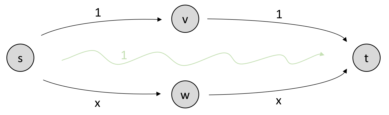
Adding artificial vertices \(V_1\) and \(V_2\) to bypass parallel edges.

As the network has polynomial edge costs, we can simply pass in the polynomial coefficients to the network constructor:

import paminco
import numpy as np

# We add artifical vertices v and w to bypass parallel edges problem
edge_data = np.array([["s", "v"],
                      ["v", "t"],
                      ["s", "w"],
                      ["w", "t"],
                      ])
# l_e = 1 = 1 + 0*x -> coeff = (1, 0)
# l_e = x = 0 + 1*x -> coeff = (0, 1)
cost = np.array([[1, 0], 
                 [1, 0],
                 [0, 1],
                 [0, 1],
                 ])
demand_data = ("s", "t", 1)
lbl2id = {"s": 0, "v": 1, "w": 2, "t": 3}
pigou = paminco.Network(edge_data=edge_data, 
                       cost_data=cost, 
                       demand_data=demand_data,
                       kw_edge={"map_labels_to_indices": lbl2id}
                       )

We find minimum cost flows that coincide with user equilibrium and system optimum if we transform the edge cost by

\[\begin{split} \begin{align} \text{User equilibrium:} \quad F_e &= \int_0^{x_e} l_e(s) ds \\ \text{System optimum:} \quad F_e &= x_e \cdot l_e. \end{align} \end{split}\]

import copy

# Calculate user equilibrium -> F_e = integral_0^(x_e) l_e(s)ds
pigou_ue = copy.deepcopy(pigou)
pigou_ue.cost.integrate(inplace=True)
fw_ue = paminco.NetworkFW(pigou_ue)
fw_ue.run()

# Calculate system optimum -> F_e = x_e * l_e
pigou_so = copy.deepcopy(pigou) 
pigou_so.cost.times_x(inplace=True)
fw_so = paminco.NetworkFW(pigou_so)
fw_so.run()

2.1 Equilibrium flows

We find flows on the (artificial) edges as:

import pandas as pd

flows_ue = fw_ue.flows[["s", "t", "x"]]
flows_so = fw_so.flows[["s", "t", "x"]]
flows = pd.merge(flows_ue, flows_so, on=["s", "t"])
flows[["s", "t"]] = pigou.shared.get_node_label(flows[["s", "t"]].values)
flows.columns = ["from", "to", "flow user eq", "flow sys opt"]
print(flows)

  from to  flow user eq  flow sys opt
0    s  v           0.0           0.5
1    v  t           0.0           0.5
2    s  w           1.0           0.5
3    w  t           1.0           0.5

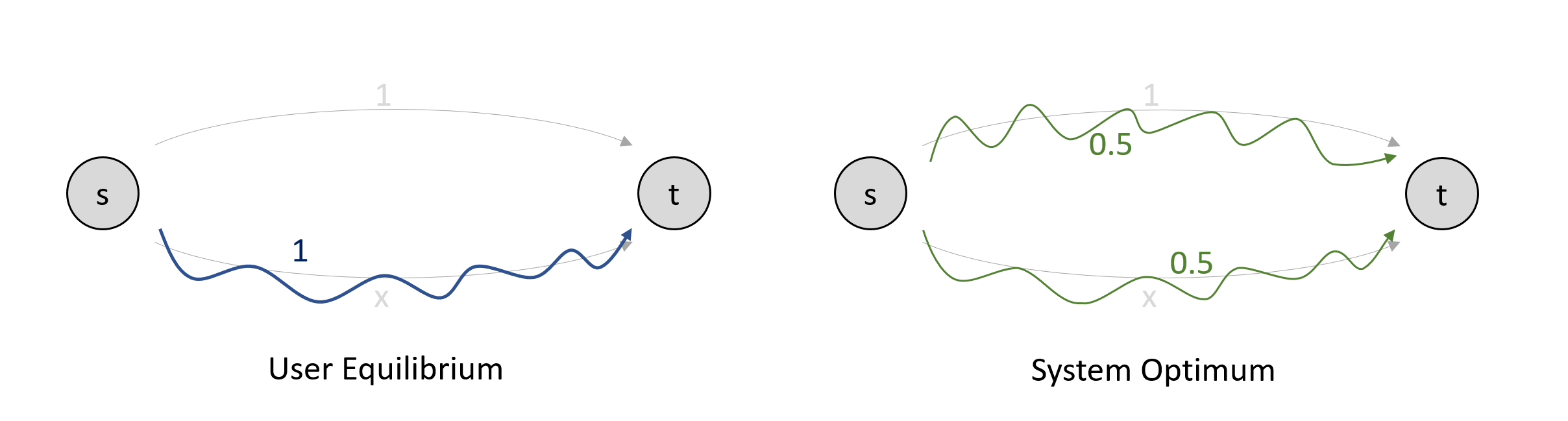
Flow in user equilibrium (left) and system optimum (right).

2.2 The Price of Anarchy

The objective function to calculate the system optimum is the total system travel time (TSTT):

\[ \begin{equation*} \text{TSTT}(\mathbf{x}) = \sum_{e \in E} x_{e} \cdot l_{e}(x_e) \end{equation*} \]

def TTST(x):
    return pigou_so.cost.F(x).sum()

We find that the total system travel time for Barcelona is increased 33.33 percent if users behave selfishly. Note that we have to scale the cost by 1/2 due to the artificial edges:

cost_ue = TTST(fw_ue.flow) / 2
cost_so = TTST(fw_so.flow) / 2
poa = cost_ue / cost_so
print("Cost user eqiulibrium: ", cost_ue)
print("Cost system optimum:   ", cost_so)
print("Price of anarchy:      ", poa.round(2))

Cost user eqiulibrium:  1.0
Cost system optimum:    0.75
Price of anarchy:       1.33