Gaslib: Gas24

Load data

We can initialize a gas network using the network and nomination XML files:

from paminco import Network 
from paminco.net import load_gas

net = load_gas("gas24")
net.size

(18, 19, 1)

where the network consists of 18 nodes and 19 edges.

Preparing the network

Set edge cost

So far, the network cost are \(F_e(x) = \beta_e x |x|\). However, as specified above, we require marginal cost \(f_e(x) = \beta_e x |x|\) to solve the minimum cost problem. Thus, before running the MCA algorithm, we have to integrate the network cost.

net.cost.integrate(inplace=True)

Set affine demand function

In the following example, we consider affine demand functions of the form:

\[ \begin{equation*} \mathbf{h}_{\text{affine}}(\lambda) = \mathbf{b}_0 + \lambda \mathbf{b}, \end{equation*} \]

where \(\mathbf{b}_0\) is a demand offset. I.e., for a demand multiplier \(\lambda=0\), the resulting demand is not zero: \(\mathbf{h}(0) \neq \mathbf{0}\). Solving this problem with MCA (and thus EFA) requires an initial phase where EFA starts in the final region of the solution of the linear problem \(\mathbf{h}(\lambda_0) = \lambda_0 \mathbf{b}_0\) with \(\lambda_0^{\text{max}} = 1\). The offset is specified by the nomination file and we set the demand direction as a commodity with single source and sink with half the rate of the offset.

demand_dir = ("entry03", "exit05", abs(net.demand()).sum())
net.set_demand((net.demand.b, demand_dir), mode="affine")

Run MCA

Finally, we run the MCA algorithm to compute parametric network flows:

from paminco import MCA
mca = MCA(net)
mca.run()

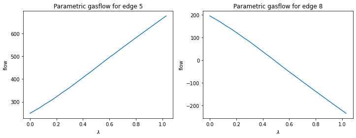
and plot the resulting parametric gas flow in the network for individual edges:

import matplotlib.pylab as plt
fig, (ax0, ax1) = plt.subplots(nrows=1, ncols=2, sharex=True, figsize=(12, 4))
d = {5: ax0, 8:ax1}
for edge, ax in d.items():
  mca.plot_flow_on_edge(edge,ax=ax)
  ax.set_xlabel("$\lambda$")
  ax.set_ylabel("flow")
  ax.set_title(f"Parametric gasflow for edge {edge}")