Parametric Minimum Cost Flows

There exists a variety of solutions to the minimum cost flow problem. paminco provides solutions to a slighly different problem.

1. Minimum cost flow functions

The goal is to find a minimum cost flow function that maps a demand factor \(\lambda\) to a minimum cost flow:

\[\begin{split}\begin{align*} \min \text { } & C(\mathbf{x}) \\ \text {s.t.} \quad \mathbf{\Gamma} \mathbf{x} &= \mathbf{h}(\lambda), \\ \mathbf{x} &\geq \mathbf{0}, \end{align*}\end{split}\]

where show definitions:

• \(\mathbf{\Gamma}\) is the incidence matrix and

• \(\mathbf{h}(\lambda): \mathbb{R} \rightarrow \mathbf{b}_{\lambda}\) a demand function.

For notational simplicity, we only discuss linear demand functions \(\mathbf{h}(\lambda) = \lambda \mathbf{b}\).

1.1 Alpha-beta-approximate minimum cost flow functions

It may not always be (computationally) feasible to compute an exact minimum cost flow function and the function has to be approximated.

Consider an interval \(\left[0, \lambda^{\max }\right]\), for which we want to find an \((\alpha, \beta)\)-approximate minimum cost flow function. A function is an \((\alpha, \beta)\)-approximate minimum cost flow function if the cost of the flow \(\mathbf{x}(\lambda)\) exceed the optimal cost at most by a relative factor of \(\alpha\) and an absolute error of \(\beta\):

\[\tilde{C}(\lambda) \leq \alpha C(\lambda)+\beta \quad \text { for all } \lambda \in\left[0, \lambda^{\max }\right],\]

where \(\tilde{C}(\lambda) = \tilde{C}(\mathbf{x}(\lambda)) = \sum_{e \in E} F_e(x_e(\lambda))\) denotes the cost of the flow \(\mathbf{x}(\lambda)\).

2. Parametric electrial flows

Instead of computing a minimum cost flow \(\mathbf{x}\) (for a fixed demand) directly, we can compute an optimal potential \(\mathbf{\pi}\) which induces a flow:

\[\begin{equation*} \mathbf{x} = \mathbf{f}^{-1} (\mathbf{\Gamma}^T \mathbf{\pi}), \end{equation*}\]

where \(\mathbf{f}^{-1}\) maps an optimal potential to an electrial flow:

\[\begin{equation*} \mathbf{f}^{-1} : \Pi \rightarrow \mathbb{R}^m \quad \mathbf{\pi} \rightarrow \mathbf{f}^{-1}(\mathbf{\pi}) := (f_e^{-1}(\pi_w - \pi_v))_{e \in E}. \end{equation*}\]

2.1 Linear marginal cost

Assume that the marginal cost for all edges are linear and of the following form: \(f_e(x) = 2ax + b\). Then we find a linear function \(\mathbf{\pi}(\lambda)\) and its induced linear electrical flow \(\mathbf{x}(\lambda)\):

\[\begin{split}\begin{align*} \mathbf{\pi}(\lambda) &= \mathbf{L}^{\ast}(\lambda \mathbf{b} + \mathbf{\Gamma} \mathbf{d}) \quad \text{and}\\ \mathbf{x}(\lambda) &= \mathbf{C} \mathbf{\Gamma}^T \mathbf{\pi}(\lambda) - \mathbf{d} = \mathbf{C} \mathbf{\Gamma}^T \mathbf{L}^{\ast}(\lambda \mathbf{b} + \mathbf{\Gamma} \mathbf{d}) - \mathbf{d} , \end{align*}\end{split}\]

where show definitions:

• \(\mathbf{C} = \text{diag}(1/2a_1, 1/2a_2, ..., 1/2a_m)\),

• \(\mathbf{d} = (b_1/2a_1, b_2/2a_2, ..., b_m/2a_m)^T\),

• \(\mathbf{L} = \mathbf{\Gamma} \mathbf{C} \mathbf{\Gamma}^T\) the weighted Laplacian of the graph, and

• \(\mathbf{L}^{\ast}\) the generalized inverse of \(\mathbf{L}\).

At a glance

Linear marginal cost result in a linear minimum cost flow function.

Example: linear resistances show / hide

Consider an electrical network with linear resistances, i.e., \(f_e(x) = r_e \cdot x\). The objective function simplifies to \(C(\mathbf{x}) = \frac{1}{2} \mathbf{x}^T \mathbf{R} \mathbf{x}\) with \(\mathbf{R} = \text{diag}(r_{e_1}, r_{e_e}, ..., r_{e_m})\).

Then we find the optimal potential and minimum cost flow as:

\[\begin{split}\begin{align*} \mathbf{\pi}(\lambda) &= \mathbf{L}^{\ast} \mathbf{h}(\lambda) \\ \mathbf{x}(\lambda) &= \mathbf{C} \mathbf{\Gamma}^T \mathbf{L}^{\ast} \mathbf{h}(\lambda), \end{align*}\end{split}\]

where \(\mathbf{C} = \mathbf{R}^{-1}\).

Thus, the parametric electrial flow is just a linear transformation of the demand function \(\mathbf{h}(\lambda)\).

2.2 Piecewise linear marginal costs

The assumption of linear marginal cost restricts the applicability of the algorithm. We now discuss problems with piecewise linear marginal costs:

Graph

Regions in \(\Pi\) and solution curve

Induced edge flows

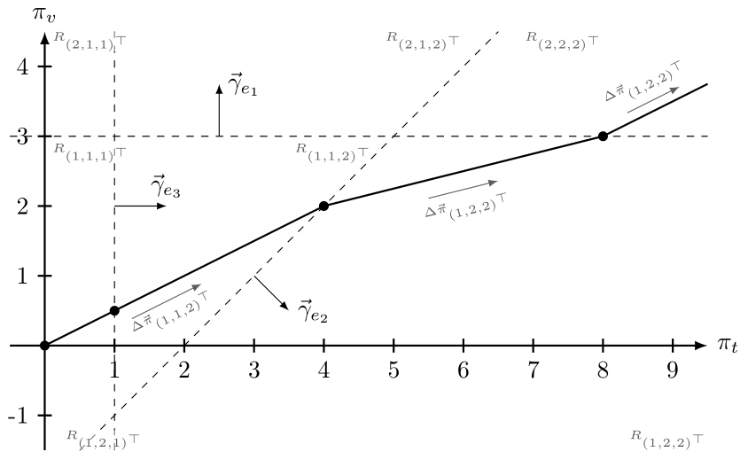
The piecewise linear marginal edge cost subdivide the potential space \(\Pi\) into regions. We denote \(\mathbf{t} = (t_{e_1}, t_{e_2}, ..., t_{e_m})^T\) the vector of the indices per edge cost function. Given an optimal potential \(\mathbf{\pi}\), the electrical flow is then:

\[\mathbf{x} = \mathbf{C}_{\mathbf{t}} \mathbf{\Gamma}^T \mathbf{\pi} - \mathbf{d}_{\mathbf{t}} = \mathbf{C}_{\mathbf{t}} \mathbf{\Gamma}^T \mathbf{L}_{\mathbf{t}}^{\ast}(\mathbf{b} + \mathbf{\Gamma} \mathbf{d}_{\mathbf{t}}) - \mathbf{d}_{\mathbf{t}}\]

In a region \(R_{\mathbf{t}}\) the solution curve is linear. The full solution curve is union of the solution segments \(\Pi_{\mathbf{t}}\) and thus a piecewise linear function:

\[\pi\left(\mathbb{R}_{\geq 0}\right):=\{\pi(\lambda) \mid \lambda \geq 0\}=\bigcup_{t \in \bar{T}} \Pi_{t}.\]

Furhter, for all regions, there exist numbers \(\lambda_t^{\text{min}}\) and \(\lambda_t^{\text{max}}\):

\[\Pi_{\mathbf{t}} = \left\{ \mathbf{\pi}_{\mathbf{t}} + \lambda \Delta \mathbf{\pi}_{\mathbf{t}} \mid \lambda \in [\lambda_t^{\text{min}}, \lambda_t^{\text{max}}] \right\} .\]

Hence, the main challenge lies in finding the correct regions \(R_{\mathbf{t}}\). The Electrial Flow Algorithm (EFA) [WK21] provides a solution for this problem.

Idea behind the Electrial Flow Algorithm

Piecewise linear marginal cost result in a subdivision of the potential space \(\Pi\). For every region \(R_{\mathbf{t}} \in \Pi\), the solution curve is linear. Thus the full solution curve is piecewise linear. The difficulty thus lies in finding the correct sequence of regions.

2.3 Interpolation of cost functions

The EFA algorithm is restricted to piecewise linear marginal cost functions \(f_e\) and thus minimum cost flow problems with piecewise quadratic cost functions. However, it is possible to approximate continous convex cost functions \(F_e\) with piecewise quadratic convex cost functions \(\tilde{F}_e\) [Roc84]. The Marginal Cost Approximation (MCA) algorithm builds on that idea and “feeds” the EFA with approximated piecewise linear marginal cost. Hence, MCA calculates an alpha-beta-approximate minimum cost flow function.

See also

MCAInterpolationRule : Criteria for proper approximation of cost functions.

References

WK21

Klimm M, Warode P (2021) “Parametric Computation of Minimum Cost Flows with Piecewise Quadratic Costs.” Mathematics of Operations Research. Available at https://www3.math.tu-berlin.de/disco/research/publications/pdf/KlimmWarode2021.pdf

Roc84

Rockafellar, RT (1984) Network Flows and Monotropic Optimization (John Wiley and Sons, Hoboken, NJ)